Where is the drill bit inside the rock?
Predicting a horizontal well's position within a stratigraphic column from gamma-ray logs alone — ROGII Wellbore Geology Prediction, a $50,000 Kaggle Featured competition with 6,191 teams. Silver medal, solo. This page includes the part I got wrong.
The problem
A horizontal well drifts vertically through a layered rock column as it is drilled. You cannot see where it is. What you get is a gamma-ray log — a one-dimensional trace of natural radioactivity along the borehole — plus the logs of every other well in the field. The task is to infer, at every point along the path, the well's true vertical position within the stratigraphy.
It is a structured sequence problem wearing a geology costume. The output is a monotone path, the evidence is a set of noisy 1D signals that must be aligned against each other, and the correct answer for one well is heavily informed by its neighbours — but only the right neighbours.
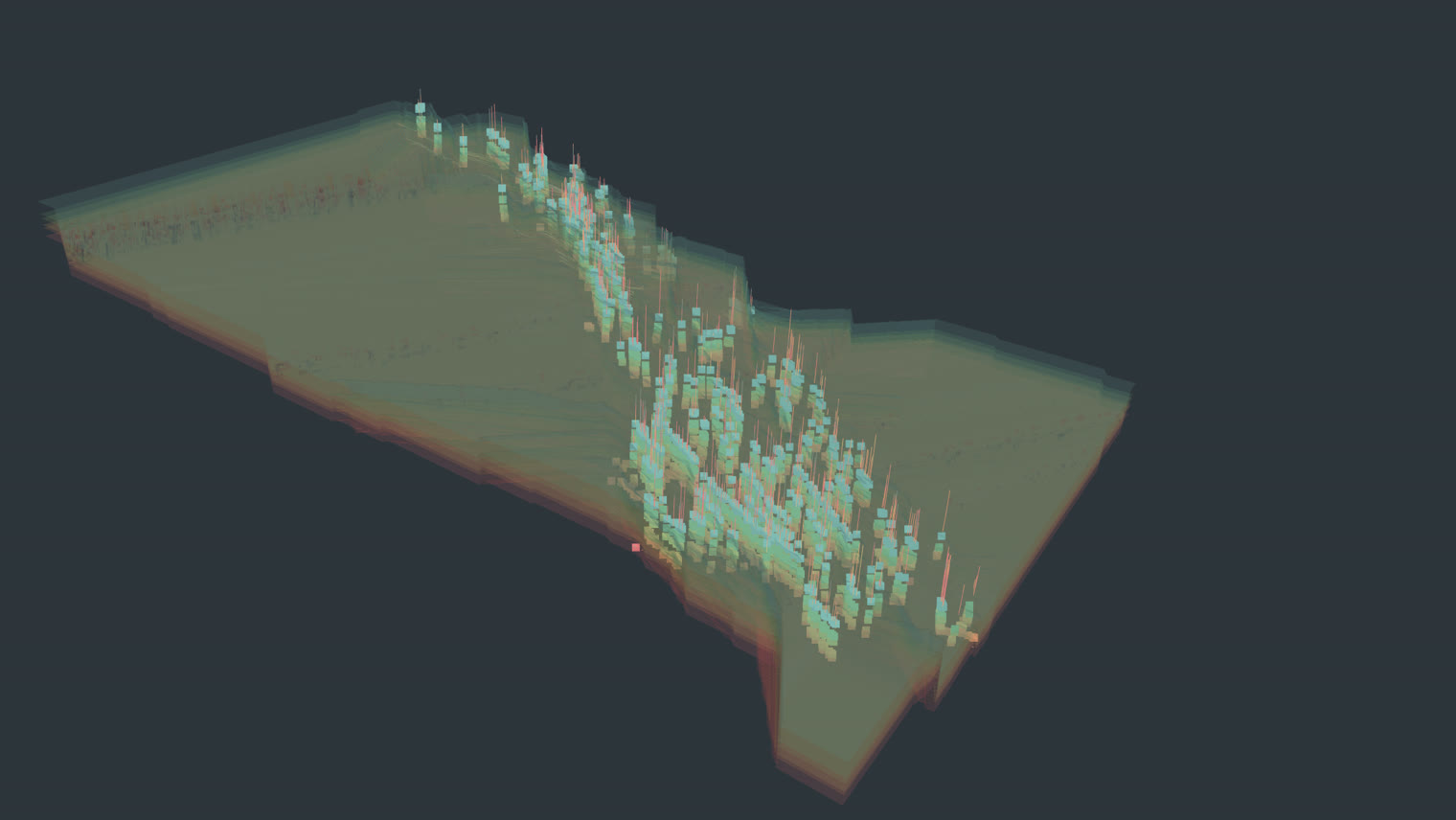
Live 3D viewer — the reconstructed subsurface
761 wells, 6 formation surfaces, and per-fold model error rendered in place. WebGL, runs in the browser.
What moved the leaderboard
Over a long campaign I kept a log of every scoring change and what caused it. The pattern that emerged was sharp enough to be worth stating plainly: nearly every large gain came from improving or conditioning the posterior before collapsing it — not from adding another model to the blend.
| Change | Public LB | Core idea |
|---|---|---|
| Structured multi-model ensemble | 8.852 → 8.265 | Heel-relative target, particle-filter / beam / NCC tracking, formation geometry |
| PG04 aligned-reference ribbon | 5.836 → 5.562 | Rank donor wells by gamma-ray profile alignment instead of geographic proximity |
| FW39 distribution-before-collapse | 6.134 → 5.877 | Pool complete seed posteriors, add geology and carrier likelihoods, then decode once |
| PGREF local pseudo-reference | 7.049 → 6.874 | Construct a better local reference log, select it through particle-filter likelihood |
| P367 graph-context selector | 7.407 → 7.257 | Use similar wells' candidate posteriors to choose among plausible paths |
| REFCARRIER02 | 6.519 → 6.393 | Treat the reference identity itself as an uncertain latent variable |
The one that mattered most
The architecture was a full-well Transformer over raw log inputs with a monotone CRF decode — about 1.1M parameters. When I first deployed it the ordinary way, blending its decoded point-path into the existing ensemble, it bought almost nothing: 6.273 → 6.224.
The gain appeared only when I stopped averaging already-decoded paths and instead kept each seed's full probability distribution alive until the very end:
- seed probability distributions from the model fleet
- + a geology unary term from fold-excluded surface consistency
- + a carrier likelihood
- → robust probability pooling
- → a single posterior-mean decode
That produced 5.877 against a deterministic matched control at 6.115 — a 0.238 improvement from the same network, purely by changing when uncertainty was discarded. The Transformer was the representation learner; the result came from preserving what it was unsure about until the final structured decision.
And the one that was almost too simple
PG04 was a one-line conceptual change. The existing code picked donor wells to correlate against by physical distance. I changed it to rank them by how well their gamma-ray profile actually aligned. That single change moved 5.836 → 5.562. All of the particle machinery I built on top of it afterwards was worth roughly a third as much combined.
The shakeup, and what I got wrong
Public 18th, private 189th. Here is the honest accounting, because I think the diagnosis is more interesting than the rank either way.
Part of it was not about me
The reshuffle hit the whole field. The team that led the public leaderboard scored 4.608 there and did not win. The eventual private winner scored 5.639 and was nowhere near the public top five. Every score degraded, and the ordering scrambled from the top down. Two splits that produce numbers that far apart, with that much rank churn between them, are not measuring the same difficulty — the private wells were drawn from a harder or simply different part of the distribution.
So some of the drop is the competition, not the competitor. But that explanation is also the comfortable one, and it does not account for all of it.
The rest of it was about me
I made 218 submissions. Every one of those was an evaluation against the public split, and every evaluation I used to decide what to keep leaked a little information from that split into my model-selection process. Two hundred and eighteen rounds of that is an enormous amount of selection pressure applied to a single, finite sample. By the end I was not choosing the model that generalised best; I was choosing the model best adapted to one particular set of held-out wells.
The irony is quite specific, and it is why this is the part of the project I actually want to talk about. The central technical lesson of the entire campaign — the thing that produced the largest single gain — was do not collapse a distribution to a point estimate before you have to. I applied that rigorously inside the model. And then I turned around and made the final decision, which submission to select, on a point estimate of generalisation: one public score, no error bars, treated as a ranking rather than as a single noisy observation.
A public leaderboard position is an estimate with a confidence interval, and on a split this size that interval is wide enough to swallow the entire distance between 18th and 189th. I knew that in the abstract. I did not act on it.
What I would do differently
- Select on cross-validation, not the public board. My local CV was the larger and more honest sample, and I let a smaller, noisier signal override it because it was attached to a visible rank.
- Measure the public/private gap as a quantity. The disagreement between CV and public score is itself data about how much a change is fitting the split rather than the problem. I logged both and never modelled the difference.
- Budget selection pressure explicitly. Treat submissions as a limited resource being spent against a finite sample, and track how much of the improvement is attributable to genuine signal versus accumulated selection.
- Prefer the robust submission when the two disagree. Where a distributionally-pooled candidate scored slightly worse publicly than a sharply tuned one, the pooled candidate was the better bet, and I had already proven that principle elsewhere in the same project.
A silver medal in a field of 6,191, working solo, is a result I am satisfied with. But the generalisation lesson is worth more to me than the two ranks would have been, and it is the thing I would carry into research work: the discipline of validating honestly matters more than the cleverness of the model, and it is much easier to preach than to practise.
Reading the viewer
The 3D page is the reconstruction, not a diagram of it — the same joint-levelled surface grid and well geometry the models consume.
- Surfaces — six formation tops, individually toggleable, opacity adjustable.
- Wells — all 761, colourable by gamma-ray bucket or by anchor/evaluation split.
- Crossing nodes — the 3,914 points where a well path crosses a formation boundary.
- Holdout inference — turn this on to draw, per cross-validation fold, the true evaluation path in aqua alongside a red ghost displaced by the model's actual error. It is a direct visual read of where the model is confident and where it drifts — and, in hindsight, exactly the kind of diagnostic I should have weighted more heavily than the public score.
Vertical exaggeration is adjustable because the real structure is nearly flat at true scale.
Try the holdout overlay
Open the viewer, tick “show predicted ghost paths”, and step through folds 1–3.
Stack
PyTorch (Transformer encoder + monotone CRF), particle filters and Rao-Blackwellised variants for path tracking, gradient-boosted trees for the tabular legs, and a cross-validated ensemble with fold-excluded geology features to avoid leakage. The viewer is three.js over exported JSON.