Turning tennis video into structured data

An end-to-end pipeline that takes raw broadcast or phone footage and produces ball trajectories, court geometry, player pose, shot events, and match statistics — run over 274 matches.

274matches processed end-to-end

0.967court keypoint val precision

4.4pxmean inlier localisation error

10,230training frames (real + synthetic)

Ball tracking across a live rally. The ball is roughly eight pixels across, moves far enough between frames to alias, and disappears behind players and against the crowd — so detection runs on a stack of consecutive frames rather than one, letting the model use motion rather than appearance alone.

The pipeline

Each video is decoded once and passed through several heads whose outputs are then fused:

Ball tracking — a TrackNet-style heatmap network over consecutive frames.
Court geometry — line and keypoint models that recover a homography from image space to real court coordinates in metres.
Player pose — per-frame skeletons for both players.
Event detection — two independent temporal heads (T-DEED and F3Set) proposing shot and point events.
Audio — an onset envelope from the soundtrack, because ball-strike and bounce are far more legible acoustically than visually.
Bounce classification — gradient-boosted and neural variants over trajectory and audio features.

Once the homography exists, everything downstream becomes geometry: in/out calls come from the bounce position and its distance to the boundary, serve speed from ball displacement in court units, and coverage from integrating player position over a point.

Pose estimation running alongside ball tracking on the same rally.

Court detection: the part that was actually hard

Ball tracking was mostly a solved recipe. Court detection was not — and it is where most of the iteration went. The court model has to fire on thin white lines under varying surfaces, lighting, and camera angles, then assign each detection the correct identity (is this the near service line or the far one?) so the homography solves.

Line-channel heatmaps

The first formulation predicts one heatmap channel per court line. Below is a single frame decomposed into its ten line channels — this is what the network actually outputs before any geometry fitting happens.

Heatmap channel activating along the far baseline — far baseline

Heatmap channel activating along the near baseline — near baseline

Heatmap channel activating along the left doubles sideline — left doubles

Heatmap channel activating along the right doubles sideline — right doubles

Heatmap channel activating along the left singles sideline — left singles

Heatmap channel activating along the right singles sideline — right singles

Heatmap channel activating along the far service line — far service

Heatmap channel activating along the near service line — near service

Heatmap channel activating along the centre service line — centre service

Heatmap channel activating along the base of the net — net ground

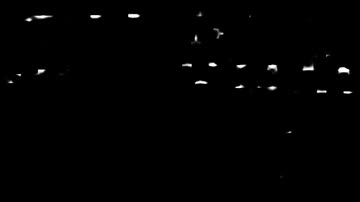
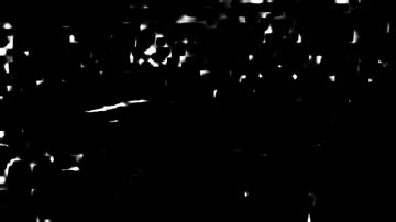
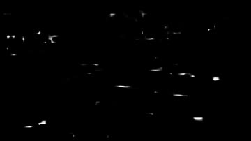
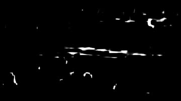
Notice how much stronger the sideline channels are than the service-line channels. Lines that are long, high-contrast and unoccluded are easy; short interior lines that players stand on are not. That imbalance drove a lot of the later work.

Detected court keypoints marked on a tennis court frame — Recovered keypoints and the fitted court model on a phone-from-the-stands frame — a deliberately hard, oblique viewpoint.

Where the architecture change paid off

The original TrackNet-style VGG U-Net could not detect the outer court corners from oblique angles at all: activations at the true corner positions sat only 1.0–1.5× above the background noise floor. No amount of post-processing recovers what the model never detected, so the fix had to be architectural — an ImageNet-pretrained backbone with a larger receptive field and skip connections.

Model	Architecture	Params	Val metric	Outer corners
TrackNet v3c	VGG U-Net, no pretraining	~13M	P = 0.683	no activation
ResNet heatmap	ResNet-18 encoder + U-Net decoder w/ skips	14.3M	P = 0.967	still weak
ResNet regression	ResNet-50 + FC coordinate head	24.7M	0.306 @ <7px	first to predict them

The pretrained backbone did not just score better, it converged far faster: precision 0.96 by epoch 4, against roughly epoch 50 for the from-scratch model. The encoder already understood edges and texture; the decoder only had to learn where to place Gaussians.

A result I had to be honest about

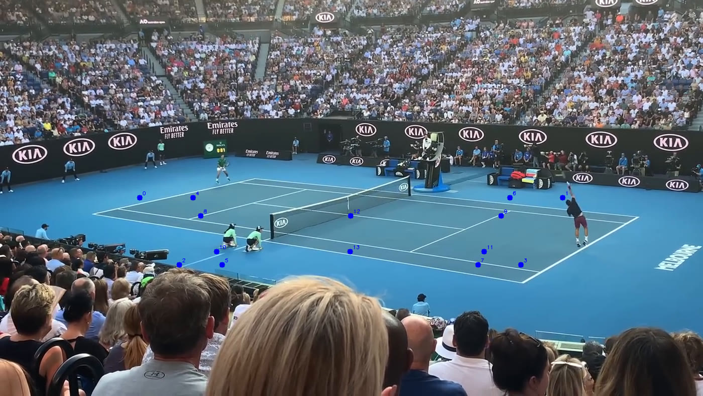
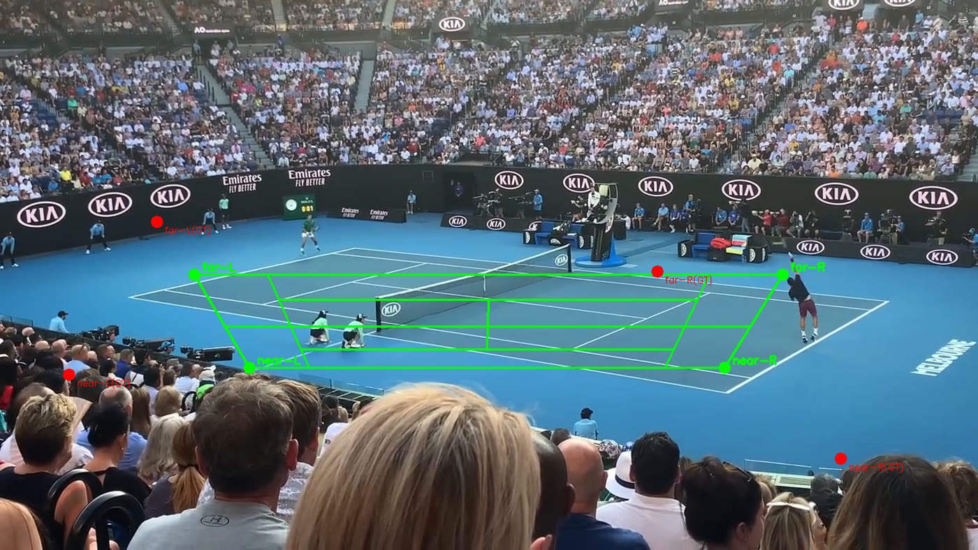
On the hard oblique frame, the heatmap model found 23 peaks, of which 12 were inliers at a 25px threshold with a mean error of 4.4px — and the overlay looks essentially correct. Yet the reported mean corner error was 609px, worse than the model it replaced.

Both numbers are real. Every inlier sat in the court interior, so the homography fitted from them extrapolates badly out to the doubles corners at the frame extremes. A metric that summarises quality at the corners will therefore punish a model that is excellent everywhere else. That is a genuine limitation of the interior-only solution, and it is also a sign the evaluation needs to separate interior fit from extrapolation rather than collapsing both into one number. Chasing the headline metric without noticing this would have sent me in exactly the wrong direction.

Side-by-side comparison of predicted versus ground-truth court corner positions — Predicted versus ground-truth corner positions — the extrapolation gap made visible.

Training data

10,230 annotated frames: 6,630 from real broadcast footage across ten matches, plus 3,600 synthetic frames rendered to imitate a phone camera from the stands. The synthetic set exists specifically to cover viewpoints the broadcast data never contains — broadcast cameras are mounted high and centred, and a model trained only on them fails immediately on amateur footage. Training ran on an RTX 5090.

What comes out

For a full match the pipeline emits per-point records — rally length, average shot depth per player, court coverage area, net approaches, recovery time between shots — plus serve analysis. On one full match it isolated 119 serves and recovered a usable velocity profile for 113 of them. Bounce events carry an in/out decision with a probability and a signed distance to the nearest boundary, so marginal calls stay marginal rather than being forced to a hard label.

Stack

PyTorch 2.7 / CUDA 12.8, ResNet backbones, CatBoost for the tabular bounce classifier, librosa-style audio onset detection, OpenCV for geometry, and a FastAPI + React review app for inspecting and correcting model output frame by frame. Containerised throughout.